Example Analysis: Avida

Preamble

This script will loosely follow the template document: it is more meant for you to get an idea of one way to approach the data processing and visualization! This analysis will primarily focus on using tidyverse tools (i.e. dplyr and ggplot).

For this dataset, the main skills we want you to practice are:

Working with multiple files: to be able to work with this data in its entirety, the files should be combined together.
Pivoting: this dataset is an example of where multiple variables are contained in the column names.

The research questions we will address are:

Easier: How does population size change over time for the wildtype (or mutant) in different medias?
Harder: How does the change in fitness over time compare between different treatment conditions and media types?

1. Load data and libraries

library(tidyverse)

wt <- read.csv("your/path/to/avida_wildtype.csv", header = TRUE, sep = ",")
mut <- read.csv("your/path/to/avida_mutant.csv", header = TRUE, sep = ",")
comp <- read.csv("your/path/to/avida_competition.csv", header = TRUE, sep = ",")

2. Format the Data

Skill: Working with multiple datasets

For this data, it will be easiest to work with them if we combine the files all together. Because they all have the same structure (same column names and number of columns), we can just use rbind() to stack the rows on top of each other.

# combine
all <- rbind(wt, mut, comp)

Other approaches to combining 3+ dataframes

A tidyverse approach to combining 3+ dataframes that share common columns/rows but are not as similar to each other could be to use reduce() and merge(). Put your dataframes into a list before combining them: reduce(list(df1, df2, df3), merge)

Skill: Pivoting

To make our data tidy, we can extract the information about media type from the population metrics columns with pivot_longer().

Because the column names are similarly structured as <media type>_<measurement>, picking the columns we want to pivot will be straightforward if we use starts_with() in the cols argument. We want to keep the measurement name that’s already in the column, so we will specify that in the names_to argument. Finally, we can use the names_sep argument to specify how to break up the current column names into the new column names (here, the new column names are all separated by the underscore).

# pivot
all <- pivot_longer(all,
                    cols = starts_with(c("minimal", "rich", "selective")),
                    names_to = c("media", ".value"), # ".value" will keep the <measurement> as the column name after pivoting
                    names_sep = "_")

3. Visualize the Data

Easier

Research question

How does population size change over time for the wildtype (or mutant) in different medias?

Since we already combined all the data, we will select the mutant/wildtype data to plot using filter() and keep them distinct with facet_wrap(). Otherwise, you can read in just the wt or mut data on their own and skip the faceting (assuming that you’ve used similar steps to pivot).

Because we want to show something changing over time, we should use a line graph.

# plot population size of the wt/mut
all |>
  filter(condition != "competition") |>
  ggplot(aes(x = update, y = pop.size, color = media)) +
  facet_wrap(~condition) +
  geom_line() +
  labs(title = "Population size of wildtype/mutant in media over time")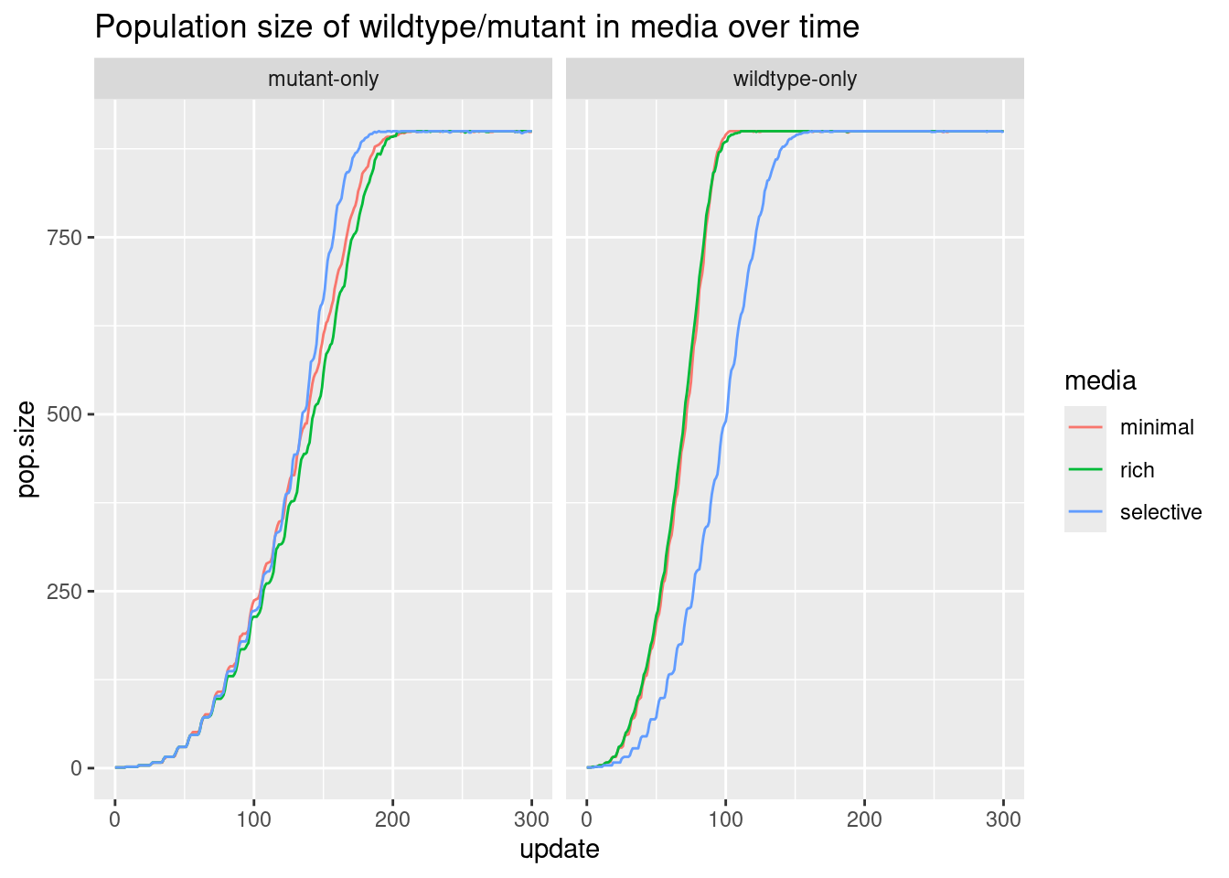

Harder

Research question

How does the change in fitness over time compare between different treatment conditions and media types?

The hardest part about this question was getting the data combined and processed: there are no further steps to take, other than to plot.

There is a similar emphasis on time here, so we will use a line plot.

# plot fitness
ggplot(all, aes(x = update, y = avg.fitness, color = condition)) +
  geom_line() +
  facet_wrap(~media) +
  labs(title = "Avg fitness of populations in media over time")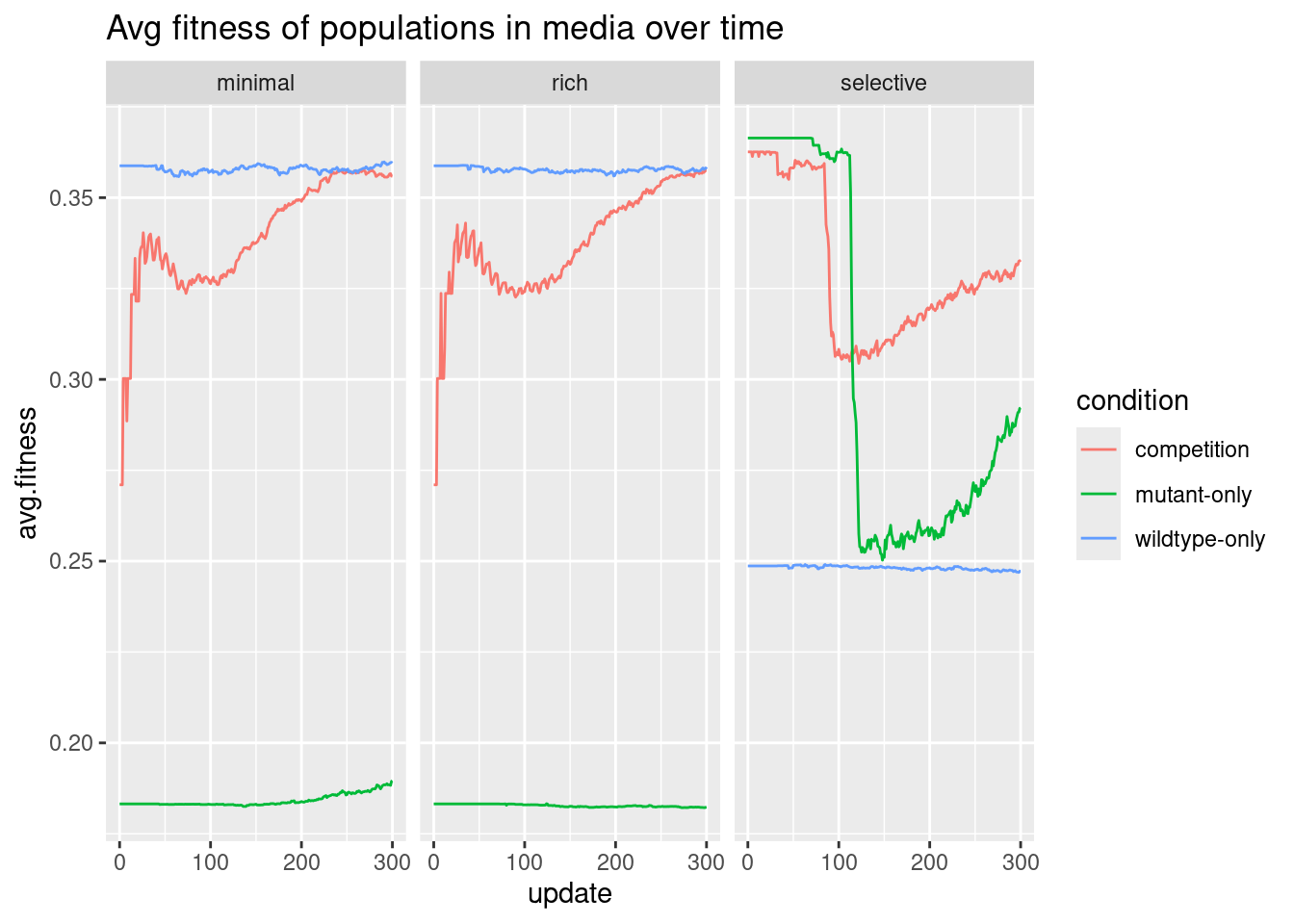

Code only

# read in data, load libraries
library(tidyverse)

wt <- read.csv("your/path/to/avida_wildtype.csv", header = TRUE, sep = ",")
mut <- read.csv("your/path/to/avida_mutant.csv", header = TRUE, sep = ",")
comp <- read.csv("your/path/to/avida_competition.csv", header = TRUE, sep = ",")

# wrangle
## combine
all <- rbind(wt, mut, comp)

## pivot
all <- pivot_longer(all,
                    cols = starts_with(c("minimal", "rich", "selective")),
                    names_to = c("media", ".value"), # ".value" will keep the <measurement> as the column name after pivoting
                    names_sep = "_")

# visualize
## easier: plot population size for wt/mut
all |>
  filter(condition != "competition") |>
  ggplot(aes(x = update, y = pop.size, color = media)) +
  facet_wrap(~condition) +
  geom_line() +
  labs(title = "Population size of wildtype/mutant in media over time")

## harder: plot fitness for all 3 conditions across all media types
ggplot(all, aes(x = update, y = avg.fitness, color = condition)) +
  geom_line() +
  facet_wrap(~media) +
  labs(title = "Avg fitness of populations in media over time")