plyxp Usage Guide

Introduction

plyxp provides efficient abstractions to the SummarizedExperiment such that using common dplyr functions feels as natural to operating on a data.frame or tibble. plyxp uses data-masking from the rlang package in order to connect dplyr functions to SummarizedExperiment slots in a manner that aims to be intuitive and avoiding ambiguity in outcomes. For more details on the design and benchmarking of plyxp, see Landis and Love (2026).

Enabling dplyr verbs

plyxp works on SummarizedExperiment objects, as well as most classes derived from this, including DESeqDataSet, SingleCellExperiment, etc.

It supports the following operations:

mutate
select
summarize
pull
filter
arrange
group_by
slice and slice_* variants

Typical use case

library(airway)
data(airway)
library(dplyr)

library(plyxp)
# to use plyxp, call `new_plyxp()` on your SummarizedExperiment object
xp <- new_plyxp(airway)

# add data (mutate) to any of the three tables,
# assay, colData, rowData,
# ...using contextual helpers cols() and rows()
xp |>
  mutate(log_counts = log1p(counts),
         cols(treated = dex == "trt"),
         rows(new_id = paste0("gene-", gene_name)))

## # A RangedSummarizedExperiment-tibble Abstraction: 63,677 × 8
##     .features      .samples | counts log_counts | gene_id gene_name gene_biotype
##     <chr>          <chr>    |  <int>      <dbl> | <chr>   <chr>     <chr>       
##   1 ENSG000000000… SRR1039… |    679       6.52 | ENSG00… TSPAN6    protein_cod…
##   2 ENSG000000000… SRR1039… |      0       0    | ENSG00… TNMD      protein_cod…
##   3 ENSG000000004… SRR1039… |    467       6.15 | ENSG00… DPM1      protein_cod…
##   4 ENSG000000004… SRR1039… |    260       5.56 | ENSG00… SCYL3     protein_cod…
##   5 ENSG000000004… SRR1039… |     60       4.11 | ENSG00… C1orf112  protein_cod…
##   …        …           …           …         …       …        …           …     
## n-4 ENSG000002734… SRR1039… |      0       0    | ENSG00… RP11-180… antisense   
## n-3 ENSG000002734… SRR1039… |      0       0    | ENSG00… TSEN34    protein_cod…
## n-2 ENSG000002734… SRR1039… |      0       0    | ENSG00… RP11-138… lincRNA     
## n-1 ENSG000002734… SRR1039… |      0       0    | ENSG00… AP000230… lincRNA     
## n   ENSG000002734… SRR1039… |      0       0    | ENSG00… RP11-80H… lincRNA     
## # ℹ n = 509,416
## # ℹ 7 more variables: new_id <chr>, `` <>, SampleName <fct>, cell <fct>,
## #   dex <fct>, albut <fct>, treated <lgl>

The operations can span contexts, and only the necessary data will be extracted from each context for computation:

# suppose a variable, `sizeFactor`, in the colData
xp$sizeFactor <- runif(8, .9, 1.1)

# we wish to scale the counts in the matrix using the size factor,
# then compute row means over the scaled counts matrix:
xp |>
  mutate(scaled_counts = counts / .cols$sizeFactor, #
         rows(ave_scl_cts = rowMeans(.assays_asis$scaled_counts)))

## # A RangedSummarizedExperiment-tibble Abstraction: 63,677 × 8
##     .features   .samples | counts scaled_counts | gene_id gene_name gene_biotype
##     <chr>       <chr>    |  <int>         <dbl> | <chr>   <chr>     <chr>       
##   1 ENSG000000… SRR1039… |    679         741.  | ENSG00… TSPAN6    protein_cod…
##   2 ENSG000000… SRR1039… |      0           0   | ENSG00… TNMD      protein_cod…
##   3 ENSG000000… SRR1039… |    467         510.  | ENSG00… DPM1      protein_cod…
##   4 ENSG000000… SRR1039… |    260         284.  | ENSG00… SCYL3     protein_cod…
##   5 ENSG000000… SRR1039… |     60          65.5 | ENSG00… C1orf112  protein_cod…
##   …      …          …           …            …       …        …           …     
## n-4 ENSG000002… SRR1039… |      0           0   | ENSG00… RP11-180… antisense   
## n-3 ENSG000002… SRR1039… |      0           0   | ENSG00… TSEN34    protein_cod…
## n-2 ENSG000002… SRR1039… |      0           0   | ENSG00… RP11-138… lincRNA     
## n-1 ENSG000002… SRR1039… |      0           0   | ENSG00… AP000230… lincRNA     
## n   ENSG000002… SRR1039… |      0           0   | ENSG00… RP11-80H… lincRNA     
## # ℹ n = 509,416
## # ℹ 7 more variables: ave_scl_cts <dbl>, `` <>, SampleName <fct>, cell <fct>,
## #   dex <fct>, albut <fct>, sizeFactor <dbl>

Calling .cols in the assay context produces an object of the matching size and orientation to the other assay data.

Alternatively we could have used purrr to compute row means:

xp |>
  mutate(scaled_counts = counts / .cols$sizeFactor,
         # You may expect a list when accessing other contexts
         # from either the rows() or cols() contexts.
         rows(ave_scl_cts = purrr::map_dbl(.assays$scaled_counts, mean)))

## # A RangedSummarizedExperiment-tibble Abstraction: 63,677 × 8
##     .features   .samples | counts scaled_counts | gene_id gene_name gene_biotype
##     <chr>       <chr>    |  <int>         <dbl> | <chr>   <chr>     <chr>       
##   1 ENSG000000… SRR1039… |    679         741.  | ENSG00… TSPAN6    protein_cod…
##   2 ENSG000000… SRR1039… |      0           0   | ENSG00… TNMD      protein_cod…
##   3 ENSG000000… SRR1039… |    467         510.  | ENSG00… DPM1      protein_cod…
##   4 ENSG000000… SRR1039… |    260         284.  | ENSG00… SCYL3     protein_cod…
##   5 ENSG000000… SRR1039… |     60          65.5 | ENSG00… C1orf112  protein_cod…
##   …      …          …           …            …       …        …           …     
## n-4 ENSG000002… SRR1039… |      0           0   | ENSG00… RP11-180… antisense   
## n-3 ENSG000002… SRR1039… |      0           0   | ENSG00… TSEN34    protein_cod…
## n-2 ENSG000002… SRR1039… |      0           0   | ENSG00… RP11-138… lincRNA     
## n-1 ENSG000002… SRR1039… |      0           0   | ENSG00… AP000230… lincRNA     
## n   ENSG000002… SRR1039… |      0           0   | ENSG00… RP11-80H… lincRNA     
## # ℹ n = 509,416
## # ℹ 7 more variables: ave_scl_cts <dbl>, `` <>, SampleName <fct>, cell <fct>,
## #   dex <fct>, albut <fct>, sizeFactor <dbl>

See below for details on how objects are made available across contexts.

plyxp also enables common grouping and summarization routines:

summary <- xp |>
  group_by(rows(gene_biotype)) |>
  summarize(col_sums = colSums(counts),
            # may rename rows with .features
            rows(.features = unique(gene_biotype)))
# summarize returns a SummarizedExperiment here,
# retaining rowData and colData

summary |> rowData()

## DataFrame with 30 rows and 1 column
##                                    gene_biotype
##                                     <character>
## protein_coding                   protein_coding
## pseudogene                           pseudogene
## processed_transcript       processed_transcript
## antisense                             antisense
## lincRNA                                 lincRNA
## ...                                         ...
## IG_C_pseudogene                 IG_C_pseudogene
## TR_D_gene                             TR_D_gene
## IG_J_pseudogene                 IG_J_pseudogene
## 3prime_overlapping_ncrna 3prime_overlapping_n..
## processed_pseudogene       processed_pseudogene

# visualizing the output as a tibble:
library(tibble)
summary |>
  pull(col_sums) |>
  as_tibble(rownames = "type")

## Warning: The `x` argument of `as_tibble.matrix()` must have unique column names if
## `.name_repair` is omitted as of tibble 2.0.0.
## ℹ Using compatibility `.name_repair`.
## This warning is displayed once per session.
## Call `lifecycle::last_lifecycle_warnings()` to see where this warning was
## generated.

## # A tibble: 30 × 9
##    type        V1       V2       V3       V4       V5       V6       V7       V8
##    <chr>    <dbl>    <dbl>    <dbl>    <dbl>    <dbl>    <dbl>    <dbl>    <dbl>
##  1 1     19413626 17741060 23926011 14360299 23003444 29233398 18114369 20103401
##  2 2       807285   733916   868950   478980   852106   946776   644006   633835
##  3 3        47547    46534    47788    26367    43965    52063    34563    35852
##  4 4        49682    43769    60098    33066    56696    66335    45654    45864
##  5 5       133335   120060   206075   125015   145078   170641   147563   149486
##  6 6         2804     2895     3417     2247     3497     4065     2508     2799
##  7 7            3        0        1        0        1        0        0        0
##  8 8            0        7        2        3        4        4        0        4
##  9 9         6038     5618     7662     5579     7869     9443     6580     6759
## 10 10        3560     3595     3963     2837     4503     5990     3320     3528
## # ℹ 20 more rows

To extract the SummarizedExperiment (if needed):

se(xp)

## class: RangedSummarizedExperiment 
## dim: 63677 8 
## metadata(1): ''
## assays(1): counts
## rownames(63677): ENSG00000000003 ENSG00000000005 ... ENSG00000273492
##   ENSG00000273493
## rowData names(3): gene_id gene_name gene_biotype
## colnames(8): SRR1039508 SRR1039509 ... SRR1039520 SRR1039521
## colData names(5): SampleName cell dex albut sizeFactor

We note that plyxp is highly related to other tidyomics projects including:

tidySummarizedExperiment
plyranges
DFplyr

Here we have focused on the design principles of: (1) function endomorphism (returning the same class of object that was input), (2) avoiding code ambiguity through strictly defined behavior and scope, and (3) allowing the user the convenience of multiple expressions for the same result, which may involve a trade-off between efficiency and verbosity.

A note on `tidySummarizedExperiment`

Some of the optimized routines in plyxp for operating on objects are called by some of the functions implemented in tidySummarizedExperiment. plyxp and tidySummarizedExperiment both provide dplyr-style interfaces to SummarizedExperiment objects, and can easily be loaded and used in the same R session without the functions conflicting. By casting objects with the new_plyxp constructor, users can enable the plyxp-driven functionality.

`plyxp` grammar

The SummarizedExperiment object contains three main components/“contexts” that we mask, the assays(), rowData()¹ and colData().

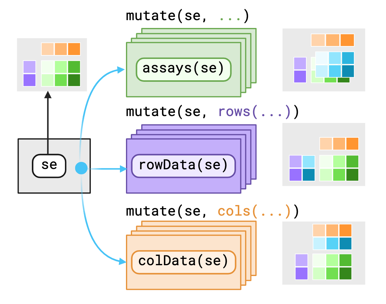
Simplified view of data masking structure. Figure made with Biorender

plyxp provides variables as-is to data within their current contexts enabling you to call S4 methods on S4 objects with dplyr verbs. If you require access to variables outside the context, you may use pronouns made available through plyxp to specify where to find those variables.

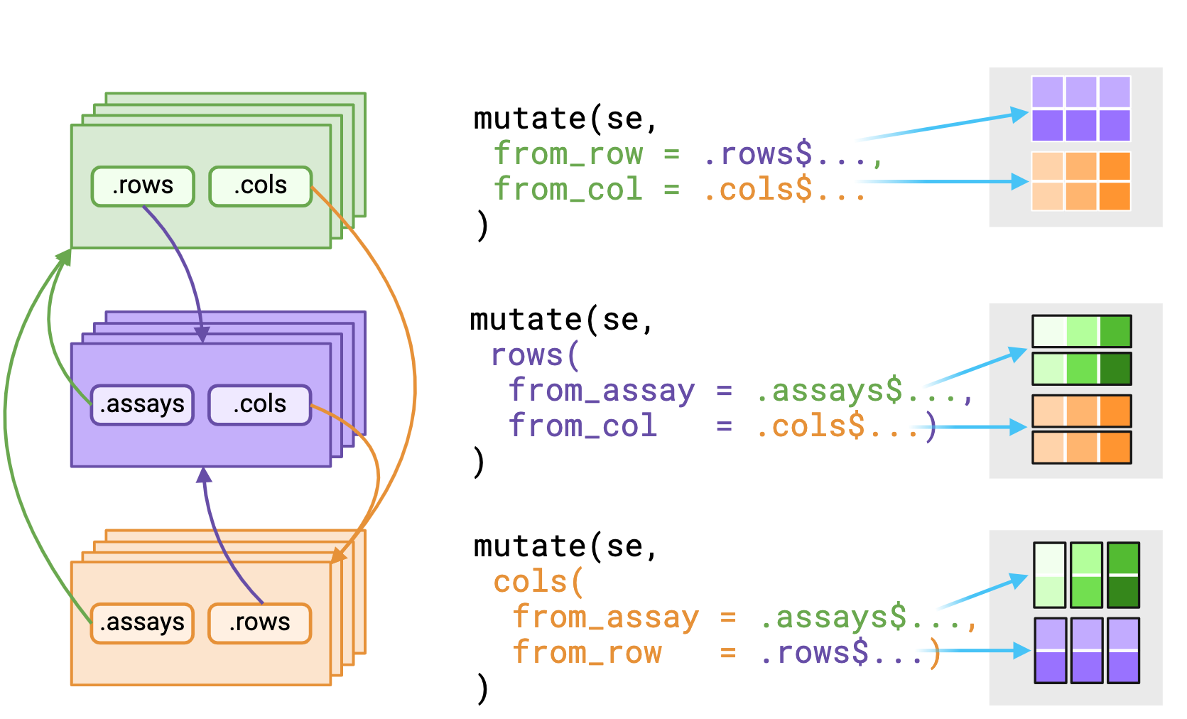
Simplified view of reshaping pronouns. Arrows indicates to where the pronoun provides access. For each pronoun listed, there is an _asis variant that returns underlying data without reshaping it to fit the context. Figure made with Biorender

The .assays, .rows and .cols pronouns outputs depends on the evaluating context. Users should expect that the underlying data returned from .rows or .cols pronouns in the assays context is a vector, replicated to match size of the assay context.

Alternatively, using a pronoun in either the rows() or cols() contexts will return a list equal in length to either nrows(rowData()) or nrows(colData()) respectively.

assay context

Default evaluation context
.assays →\to contextual pronoun, returns list of the matrix, sliced by the dimension it was referenced from.
- within the rowData context: .assays$foo is an alias for lapply(seq_len(nrow()), \(i, x) x[i,,drop=FALSE], x = foo)
- within the colData context: .assays$foo is an alias for lapply(seq_len(ncol()), \(i, x) x[,i,drop=FALSE], x = foo)
.assays_asis $\to$ pronoun to direct bindings in assays()
assay_ctx(expr, asis = FALSE) $\to$ short hand to bind the assay context in front of the current context.

rows context

rows(...) $\to$ sentinel function call to indicate evaluation context.
.rows →\to contextual pronoun
- within assay context: .rows$foo is an alias for vctrs::vec_rep(foo, times = ncol())
- within colData context: .rows$foo is an alias for vctrs::vec_rep(list(foo), times = n())
.rows_asis $\to$ pronoun to direct bindings in rowData()
row_ctx(expr, asis = FALSE) $\to$ shorthand to bind the rowData context in front of the current context

cols context

cols(...) $\to$ sentinel function call to indicate evaluation context.
.cols →\to contextual pronoun
- within assay context: .cols$foo is an alias for vctrs::vec_rep_each(foo, times = nrow())
- within rowData context: .rows$foo is an alias for vctrs::vec_rep(list(foo), times = n())
.cols_asis $\to$ pronoun to direct bindings in colData()
col_ctx(expr, asis = FALSE) $\to$ shorthand to bind the colData context in front of the current context

Multiple equivalent expressions

We can compare two ways of dividing out a vector from colData along the columns of assay data:

# here the `.cols$` pronoun reshapes the data to fit the `assays` context
xp |>
  mutate(scaled_counts = counts / .cols$sizeFactor)

## # A RangedSummarizedExperiment-tibble Abstraction: 63,677 × 8
##     .features .samples | counts scaled_counts | gene_id gene_name gene_biotype |
##     <chr>     <chr>    |  <int>         <dbl> | <chr>   <chr>     <chr>        |
##   1 ENSG0000… SRR1039… |    679         741.  | ENSG00… TSPAN6    protein_cod… |
##   2 ENSG0000… SRR1039… |      0           0   | ENSG00… TNMD      protein_cod… |
##   3 ENSG0000… SRR1039… |    467         510.  | ENSG00… DPM1      protein_cod… |
##   4 ENSG0000… SRR1039… |    260         284.  | ENSG00… SCYL3     protein_cod… |
##   5 ENSG0000… SRR1039… |     60          65.5 | ENSG00… C1orf112  protein_cod… |
##   …     …         …           …            …       …        …           …       
## n-4 ENSG0000… SRR1039… |      0           0   | ENSG00… RP11-180… antisense    |
## n-3 ENSG0000… SRR1039… |      0           0   | ENSG00… TSEN34    protein_cod… |
## n-2 ENSG0000… SRR1039… |      0           0   | ENSG00… RP11-138… lincRNA      |
## n-1 ENSG0000… SRR1039… |      0           0   | ENSG00… AP000230… lincRNA      |
## n   ENSG0000… SRR1039… |      0           0   | ENSG00… RP11-80H… lincRNA      |
## # ℹ n = 509,416
## # ℹ 5 more variables: SampleName <fct>, cell <fct>, dex <fct>, albut <fct>,
## #   sizeFactor <dbl>

# this is equivalent to the following, where we have to transpose
# the `counts` assay data twice to enable the correct recycling
# of the size factor vector
xp |>
  mutate(scaled_counts = t(t(counts) / .cols_asis$sizeFactor))

## # A RangedSummarizedExperiment-tibble Abstraction: 63,677 × 8
##     .features .samples | counts scaled_counts | gene_id gene_name gene_biotype |
##     <chr>     <chr>    |  <int>         <dbl> | <chr>   <chr>     <chr>        |
##   1 ENSG0000… SRR1039… |    679         741.  | ENSG00… TSPAN6    protein_cod… |
##   2 ENSG0000… SRR1039… |      0           0   | ENSG00… TNMD      protein_cod… |
##   3 ENSG0000… SRR1039… |    467         510.  | ENSG00… DPM1      protein_cod… |
##   4 ENSG0000… SRR1039… |    260         284.  | ENSG00… SCYL3     protein_cod… |
##   5 ENSG0000… SRR1039… |     60          65.5 | ENSG00… C1orf112  protein_cod… |
##   …     …         …           …            …       …        …           …       
## n-4 ENSG0000… SRR1039… |      0           0   | ENSG00… RP11-180… antisense    |
## n-3 ENSG0000… SRR1039… |      0           0   | ENSG00… TSEN34    protein_cod… |
## n-2 ENSG0000… SRR1039… |      0           0   | ENSG00… RP11-138… lincRNA      |
## n-1 ENSG0000… SRR1039… |      0           0   | ENSG00… AP000230… lincRNA      |
## n   ENSG0000… SRR1039… |      0           0   | ENSG00… RP11-80H… lincRNA      |
## # ℹ n = 509,416
## # ℹ 5 more variables: SampleName <fct>, cell <fct>, dex <fct>, albut <fct>,
## #   sizeFactor <dbl>

Advanced features

Object integrity

plyxp provides an opinionated framework for how dplyr verbs should interact with SummarizedExperiment objects. In general, plyxp will not allow any operations that it could not guarantee a valid return object.

It is for this reason that arrange(), filter() and group_by() do not allow operations in the default assay context, as this would likely break the assumed structure of a SummarizedExperiment object.

Grouping

plyxp also supports group_by operations allowing users to query information with dplyr::n() or dplyr::cur_group_id(). However due to the linked structure of a SummarizedExperiment object and plyxp providing multiple evaluation contexts, grouping operations would be complex and return values would be potentionally ambiguous.

It is for this reason that groupings are themselves contextual. The assay context is dependently linked to both the groupings of the rows and cols contexts but, the grouping of rows is ignored when viewed from the cols context and similarly the grouping of cols is ignored when viewed from the rows context. In this way, we have chosen to make the groupings of rows and cols independent between each other. The below figure attempts to show how groupings are conditionally dropped for the scope of an evaluation.

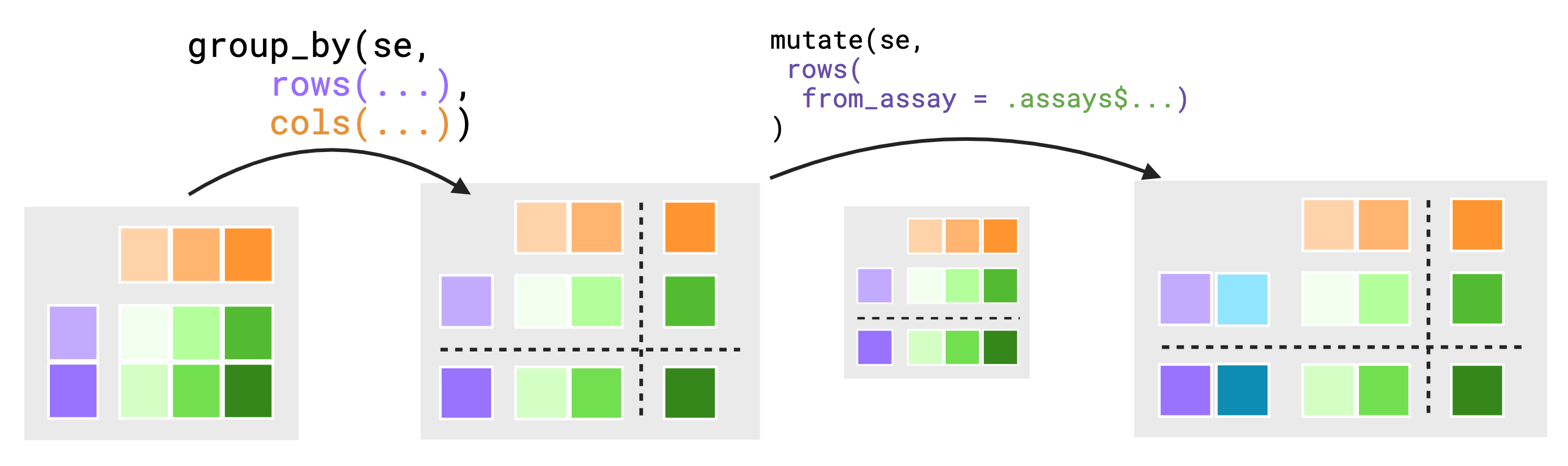
When evaluating in row context, groupings along colData() are temporarily ignored. Figure created with Biorender

To further motivate this choice, suppose we did not drop grouping values. Assume you have a small 5 by 4 SummarizedExperiment object. Both of the rowData() and colData() are grouped such that there are 2 groups in both rowData() and colData() totaling in 4 groups across the assays.

group_by(se_simple, rows(direction), cols(condition)) |>
  mutate(rows(data_from_cols = .cols$condition))

The above syntax implies we wish to move data from the colData() into the rowData(). From a previously established conventions, we would expect the output to be an alias for vctrs::vec_rep(list(condition), times = n()).
Additionally the rows() sentinal will expect that the output of .cols$condition will need to match the size of the evaluation context.

Unfortunately, this becomes extremely difficult to resolve with the current conventions. Without dropping the cols() groupings, each rows() grouping is evaluated equal to the number of groups in cols(). At first glance, this may seem desirable, but the problem arises when considering how theses outputs across groups should be stored per group of rows(). For example, should the output of the .cols$condition return a list equal to the number of groups of the column context? If yes, we would need to consider the size stability of the output context! Assuming that rowData() has at least one group with three elements, there is no guarentee it would fit (this also makes a poor assumption that the elements of rowData() somehow correspond to the groups of colData()). Thus we would be left with wrapping all the results in a list and replicating to the appropriate size. When its all said and done, we would have a list of lists, which is difficult to reason about, potentionally unexpected and painful to work with. For this reason the only groupings present in the rowData() context are the groupings in rowData(), and similarly for the colData() context.

Slicing

plyxp supports slice() and its convenience variants slice_head(), slice_tail(), slice_min(), slice_max() and slice_sample(). Unlike their data.frame counterparts, these verbs use the rows() and cols() context functions to declare which dimension(s) of the object to slice. The assay context is not available for slicing, as removing individual cells of an assay would break the structure of the object.

slice() takes integer positions:

xp |>
  slice(rows(1:5), cols(c(1, 3)))

## # A RangedSummarizedExperiment-tibble Abstraction: 5 × 2
##    .features     .samples | counts | gene_id gene_name gene_biotype | SampleName
##    <chr>         <chr>    |  <int> | <chr>   <chr>     <chr>        | <fct>     
##  1 ENSG00000000… SRR1039… |    679 | ENSG00… TSPAN6    protein_cod… | GSM1275862
##  2 ENSG00000000… SRR1039… |      0 | ENSG00… TNMD      protein_cod… | GSM1275862
##  3 ENSG00000000… SRR1039… |    467 | ENSG00… DPM1      protein_cod… | GSM1275862
##  4 ENSG00000000… SRR1039… |    260 | ENSG00… SCYL3     protein_cod… | GSM1275862
##  5 ENSG00000000… SRR1039… |     60 | ENSG00… C1orf112  protein_cod… | GSM1275862
##  6 ENSG00000000… SRR1039… |    873 | ENSG00… TSPAN6    protein_cod… | GSM1275866
##  7 ENSG00000000… SRR1039… |      0 | ENSG00… TNMD      protein_cod… | GSM1275866
##  8 ENSG00000000… SRR1039… |    621 | ENSG00… DPM1      protein_cod… | GSM1275866
##  9 ENSG00000000… SRR1039… |    263 | ENSG00… SCYL3     protein_cod… | GSM1275866
## 10 ENSG00000000… SRR1039… |     40 | ENSG00… C1orf112  protein_cod… | GSM1275866
## # ℹ 4 more variables: cell <fct>, dex <fct>, albut <fct>, sizeFactor <dbl>

For slice_head() and slice_tail(), the contexts must be empty, and only indicate which dimension(s) to slice:

xp |>
  slice_head(rows(), cols(), n = 3)

## # A RangedSummarizedExperiment-tibble Abstraction: 3 × 3
##   .features      .samples | counts | gene_id gene_name gene_biotype | SampleName
##   <chr>          <chr>    |  <int> | <chr>   <chr>     <chr>        | <fct>     
## 1 ENSG000000000… SRR1039… |    679 | ENSG00… TSPAN6    protein_cod… | GSM1275862
## 2 ENSG000000000… SRR1039… |      0 | ENSG00… TNMD      protein_cod… | GSM1275862
## 3 ENSG000000004… SRR1039… |    467 | ENSG00… DPM1      protein_cod… | GSM1275862
## 4 ENSG000000000… SRR1039… |    448 | ENSG00… TSPAN6    protein_cod… | GSM1275863
## 5 ENSG000000000… SRR1039… |      0 | ENSG00… TNMD      protein_cod… | GSM1275863
## 6 ENSG000000004… SRR1039… |    515 | ENSG00… DPM1      protein_cod… | GSM1275863
## 7 ENSG000000000… SRR1039… |    873 | ENSG00… TSPAN6    protein_cod… | GSM1275866
## 8 ENSG000000000… SRR1039… |      0 | ENSG00… TNMD      protein_cod… | GSM1275866
## 9 ENSG000000004… SRR1039… |    621 | ENSG00… DPM1      protein_cod… | GSM1275866
## # ℹ 4 more variables: cell <fct>, dex <fct>, albut <fct>, sizeFactor <dbl>

xp |>
  slice_tail(cols(), n = 2) |>
  colData()

## DataFrame with 2 rows and 5 columns
##            SampleName     cell      dex    albut sizeFactor
##              <factor> <factor> <factor> <factor>  <numeric>
## SRR1039520 GSM1275874  N061011    untrt    untrt   0.999555
## SRR1039521 GSM1275875  N061011    trt      untrt   0.957953

slice_min() and slice_max() order by a variable within a context. Here we compute the average count per gene, and keep the five most highly expressed genes:

xp_ave <- xp |>
  mutate(rows(ave_count = rowMeans(.assays_asis$counts)))

xp_ave |>
  slice_max(rows(ave_count), n = 5) |>
  rowData()

## DataFrame with 5 rows and 4 columns
##                         gene_id   gene_name   gene_biotype ave_count
##                     <character> <character>    <character> <numeric>
## ENSG00000115414 ENSG00000115414         FN1 protein_coding    328813
## ENSG00000011465 ENSG00000011465         DCN protein_coding    300740
## ENSG00000198804 ENSG00000198804      MT-CO1 protein_coding    267427
## ENSG00000156508 ENSG00000156508      EEF1A1 protein_coding    260605
## ENSG00000164692 ENSG00000164692      COL1A2 protein_coding    209321

Slicing respects groupings within each context, so we can find the top genes per biotype, or the sample with the smallest library size per treatment:

xp_ave |>
  filter(rows(gene_biotype %in% c("protein_coding", "lincRNA"))) |>
  group_by(rows(gene_biotype)) |>
  slice_max(rows(ave_count), n = 3) |>
  rowData()

## DataFrame with 6 rows and 4 columns
##                   gene_biotype         gene_id     gene_name ave_count
##                    <character>     <character>   <character> <numeric>
## ENSG00000115414 protein_coding ENSG00000115414           FN1 328812.62
## ENSG00000011465 protein_coding ENSG00000011465           DCN 300740.00
## ENSG00000198804 protein_coding ENSG00000198804        MT-CO1 267426.88
## ENSG00000272761        lincRNA ENSG00000272761 RP11-572C15.6  35348.00
## ENSG00000245532        lincRNA ENSG00000245532         NEAT1  25066.50
## ENSG00000214548        lincRNA ENSG00000214548          MEG3   9949.38

xp |>
  mutate(cols(lib_size = colSums(.assays_asis$counts))) |>
  group_by(cols(dex)) |>
  slice_min(cols(lib_size), n = 1) |>
  colData()

## DataFrame with 2 rows and 6 columns
##                 dex SampleName     cell    albut sizeFactor  lib_size
##            <factor>   <factor> <factor> <factor>  <numeric> <numeric>
## SRR1039520    untrt GSM1275874  N061011    untrt   0.999555  19126151
## SRR1039513    trt   GSM1275867  N052611    untrt   0.931442  15163415

slice_sample() randomly samples rows and/or columns. An empty context indicates a uniform sample, while a non-empty context (or the weight_by argument) supplies sampling weights. Here we take two samples per treatment group, and separately, a sample of genes weighted by their average count:

set.seed(1)
xp |>
  group_by(cols(dex)) |>
  slice_sample(cols(), n = 2) |>
  colData()

## DataFrame with 4 rows and 5 columns
##                 dex SampleName     cell    albut sizeFactor
##            <factor>   <factor> <factor> <factor>  <numeric>
## SRR1039508    untrt GSM1275862  N61311     untrt   0.916150
## SRR1039516    untrt GSM1275870  N080611    untrt   0.901480
## SRR1039509    trt   GSM1275863  N61311     untrt   1.066867
## SRR1039513    trt   GSM1275867  N052611    untrt   0.931442

xp_ave |>
  slice_sample(weight_by = rows(ave_count), n = 5) |>
  rowData()

## DataFrame with 5 rows and 4 columns
##                         gene_id   gene_name   gene_biotype  ave_count
##                     <character> <character>    <character>  <numeric>
## ENSG00000110697 ENSG00000110697     PITPNM1 protein_coding    699.250
## ENSG00000100865 ENSG00000100865        CINP protein_coding    419.125
## ENSG00000117394 ENSG00000117394      SLC2A1 protein_coding   2770.125
## ENSG00000136448 ENSG00000136448        NMT1 protein_coding   3164.250
## ENSG00000164692 ENSG00000164692      COL1A2 protein_coding 209320.625

Note that n (or prop) should always be passed by name. Due to argument checks in the dplyr generics, some calls will error otherwise, e.g. slice_head(xp, rows()) or slice_min(xp, rows(foo), cols(bar)). See ?slice_extras for more details.

Printing

Motivated by the show/print function in tidySummarizedExperiment, we visualize the data as if it was tabular. plyxp offers the option to opt-in on this behavior by setting the associated global option:

options("show_SummarizedExperiment_as_tibble_abstraction" = TRUE)

Alternatively, you may use helper functions use_show_tidy() and use_show_default() to enable and disable this alternative printing respectively.

Since plyxp aims to leave the input data as-is when possible, we have considered providing support for printing S4Vectors within a tibble(). To be clear, plyxp will not allow you to put S4Vectors inside a tibble(), but will allow for S4Vectors to be printed with pillar(), the formatting engine behind tibble() pretty printing.

To enable this behavior, before any data is reported to the user, we proxy any S4Vector with a custom vctrs_vctr object with plyxp::vec_phantom(). In truth, the vec_phantom object is a simple integer vector with a “phantomData” attribute. This allows us to carry along S4Vector through pillar()’s printing pipeline until it is time to print the column.

The pillar_shaft() method for vec_phantom will format the S4 data with plyxp_pillar_format() generic, which by default calls S4Vectors::showAsCell(). Users are free to create their own methods for S4 vectors that differ from S4Vectors::showAsCell() if they like, as seen in ?`plyxp-printing`

Renaming rows or columns

Inspired by tidySummarizedExperiment, plyxp provides access to the rownames and colnames of a SummarizedExperiment object by installing .features and .samples into the rowData() and colData() contexts respectively. These are special in that assigning a value to .features in the rowData() context or .samples in the colData() context does not create a new column, but changes the rownames or colnames of the resulting object.

se_simple

## # A SummarizedExperiment-tibble Abstraction: 5 × 4
##     .features .samples | counts logcounts | gene  length direction | sample
##     <chr>     <chr>    |  <int>     <dbl> | <chr>  <int> <chr>     | <chr> 
##   1 row_1     col_1    |     14      2.64 | g1         1 -         | s1    
##   2 row_2     col_1    |     19      2.94 | g2        24 +         | s1    
##   3 row_3     col_1    |     16      2.77 | g3        60 +         | s1    
##   4 row_4     col_1    |     11      2.40 | g4        39 -         | s1    
##   5 row_5     col_1    |     18      2.89 | g5        37 +         | s1    
##   …   …         …             …        …     …         … …            …    
## n-4 row_1     col_4    |      9      2.20 | g1         1 -         | s4    
## n-3 row_2     col_4    |      4      1.39 | g2        24 +         | s4    
## n-2 row_3     col_4    |     20      3.00 | g3        60 +         | s4    
## n-1 row_4     col_4    |      3      1.10 | g4        39 -         | s4    
## n   row_5     col_4    |      5      1.61 | g5        37 +         | s4    
## # ℹ n = 20
## # ℹ 1 more variable: condition <chr>

# moving data to rownames and colnames
se_simple |>
  mutate(
    orig_names = sprintf(
      "%s-%s",
      # .features is installed in the rows() context
      .rows$.features,
      # .samples is installed in the cols() context
      .cols$.samples),
    rows(.features = gene,
         # deleting rowData column
         gene = NULL),
    cols(.samples = sample,
         # deleting colData column
         sample = NULL)
  )

## # A SummarizedExperiment-tibble Abstraction: 5 × 4
##     .features .samples | counts logcounts orig_names  | length direction |
##     <chr>     <chr>    |  <int>     <dbl> <chr>       |  <int> <chr>     |
##   1 g1        s1       |     14      2.64 row_1-col_1 |      1 -         |
##   2 g2        s1       |     19      2.94 row_2-col_1 |     24 +         |
##   3 g3        s1       |     16      2.77 row_3-col_1 |     60 +         |
##   4 g4        s1       |     11      2.40 row_4-col_1 |     39 -         |
##   5 g5        s1       |     18      2.89 row_5-col_1 |     37 +         |
##   …  …         …              …        …       …             … …          
## n-4 g1        s4       |      9      2.20 row_1-col_4 |      1 -         |
## n-3 g2        s4       |      4      1.39 row_2-col_4 |     24 +         |
## n-2 g3        s4       |     20      3.00 row_3-col_4 |     60 +         |
## n-1 g4        s4       |      3      1.10 row_4-col_4 |     39 -         |
## n   g5        s4       |      5      1.61 row_5-col_4 |     37 +         |
## # ℹ n = 20
## # ℹ 1 more variable: condition <chr>

Best practices

There is some overhead in creating the evaluation mask per dplyr verb. It is recommended to try to reduce the number of dplyr verb calls and instead increase the content of each verb. For example instead of doing:

.data |>
  mutate(foo = bar) |>
  mutate(baz = foo^2)

do the following:

.data |>
  mutate(
    foo = bar,
    baz = foo^2
  )

Community and support

Please feel free to post questions about plyxp to:

the Bioconductor support site
as an Issue on GitHub
in the #tidiness_in_bioc channel on the community-bioc Slack

For code contributions:

For small fixes, feel free to post a PR on GitHub
For larger structural changes to the package code, please reach out to the development team first through one of the above channels.

Thanks for your interest in plyxp!

Session info

devtools::session_info()

## ─ Session info ───────────────────────────────────────────────────────────────
##  setting  value
##  version  R version 4.5.2 (2025-10-31)
##  os       Ubuntu 24.04.3 LTS
##  system   x86_64, linux-gnu
##  ui       X11
##  language en
##  collate  en_US.UTF-8
##  ctype    en_US.UTF-8
##  tz       UTC
##  date     2026-11-05
##  pandoc   3.8.2.1 @ /usr/bin/ (via rmarkdown)
##  quarto   1.7.32 @ /usr/local/bin/quarto
## 
## ─ Packages ───────────────────────────────────────────────────────────────────
##  package              * version date (UTC) lib source
##  abind                  1.4-8   2024-09-12 [1] RSPM (R 4.5.0)
##  airway               * 1.30.0  2025-10-30 [1] Bioconductor 3.22 (R 4.5.2)
##  Biobase              * 2.70.0  2025-10-29 [1] Bioconductor 3.22 (R 4.5.2)
##  BiocGenerics         * 0.56.0  2025-10-29 [1] Bioconductor 3.22 (R 4.5.2)
##  bslib                  0.12.0  2026-08-04 [2] RSPM (R 4.5.0)
##  cachem                 1.1.0   2024-05-16 [2] RSPM (R 4.5.0)
##  cli                    3.6.6   2026-04-09 [2] RSPM (R 4.5.0)
##  DelayedArray           0.36.1  2026-03-31 [1] Bioconductor 3.22 (R 4.5.2)
##  desc                   1.4.3   2023-12-10 [2] RSPM (R 4.5.0)
##  devtools               2.5.2   2026-04-30 [2] RSPM (R 4.5.0)
##  digest                 0.6.39  2025-11-19 [2] RSPM (R 4.5.0)
##  dplyr                * 1.2.1   2026-04-03 [1] RSPM (R 4.5.0)
##  ellipsis               0.3.3   2026-04-04 [2] RSPM (R 4.5.0)
##  evaluate               1.0.5   2025-08-27 [2] RSPM (R 4.5.0)
##  fastmap                1.2.0   2024-05-15 [2] RSPM (R 4.5.0)
##  fs                     2.1.0   2026-04-18 [2] RSPM (R 4.5.0)
##  generics             * 0.1.4   2025-05-09 [1] RSPM (R 4.5.0)
##  GenomicRanges        * 1.62.1  2025-12-08 [1] Bioconductor 3.22 (R 4.5.2)
##  glue                   1.8.1   2026-04-17 [2] RSPM (R 4.5.0)
##  htmltools              0.5.9   2025-12-04 [2] RSPM (R 4.5.0)
##  htmlwidgets            1.6.4   2023-12-06 [2] RSPM (R 4.5.0)
##  IRanges              * 2.44.0  2025-10-29 [1] Bioconductor 3.22 (R 4.5.2)
##  jquerylib              0.1.4   2021-04-26 [2] RSPM (R 4.5.0)
##  jsonlite               2.0.0   2025-03-27 [2] RSPM (R 4.5.0)
##  knitr                  1.52    2026-09-06 [2] RSPM (R 4.5.0)
##  lattice                0.23-1  2026-08-12 [3] RSPM (R 4.5.0)
##  lifecycle              1.0.5   2026-01-08 [2] RSPM (R 4.5.0)
##  magrittr               2.0.5   2026-04-04 [2] RSPM (R 4.5.0)
##  Matrix                 1.7-6   2026-07-25 [3] RSPM (R 4.5.0)
##  MatrixGenerics       * 1.22.0  2025-10-29 [1] Bioconductor 3.22 (R 4.5.2)
##  matrixStats          * 1.5.0   2025-01-07 [1] RSPM (R 4.5.0)
##  memoise                2.0.1   2021-11-26 [2] RSPM (R 4.5.0)
##  otel                   0.2.0   2025-08-29 [2] RSPM (R 4.5.0)
##  pillar                 1.11.1  2025-09-17 [2] RSPM (R 4.5.0)
##  pkgbuild               1.4.8   2025-05-26 [2] RSPM (R 4.5.0)
##  pkgconfig              2.0.3   2019-09-22 [2] RSPM (R 4.5.0)
##  pkgdown                2.2.1   2026-07-07 [2] RSPM (R 4.5.0)
##  pkgload                1.5.3   2026-06-15 [2] RSPM (R 4.5.0)
##  plyxp                * 1.7.8   2026-11-05 [1] Bioconductor
##  purrr                  1.2.2   2026-04-10 [2] RSPM (R 4.5.0)
##  R6                     2.6.1   2025-02-15 [2] RSPM (R 4.5.0)
##  ragg                   1.5.2   2026-03-23 [2] RSPM (R 4.5.0)
##  rlang                  1.3.0   2026-07-05 [2] RSPM (R 4.5.0)
##  rmarkdown              2.32    2026-09-01 [2] RSPM (R 4.5.0)
##  S4Arrays               1.10.1  2025-12-01 [1] Bioconductor 3.22 (R 4.5.2)
##  S4Vectors            * 0.48.1  2026-04-05 [1] Bioconductor 3.22 (R 4.5.2)
##  S7                     0.2.2   2026-04-22 [1] RSPM (R 4.5.0)
##  sass                   0.4.10  2025-04-11 [2] RSPM (R 4.5.0)
##  Seqinfo              * 1.0.0   2025-10-29 [1] Bioconductor 3.22 (R 4.5.2)
##  sessioninfo            1.2.4   2026-06-04 [2] RSPM (R 4.5.0)
##  SparseArray            1.10.10 2026-03-30 [1] Bioconductor 3.22 (R 4.5.2)
##  SummarizedExperiment * 1.40.0  2025-10-29 [1] Bioconductor 3.22 (R 4.5.2)
##  systemfonts            1.3.2   2026-03-05 [2] RSPM (R 4.5.0)
##  textshaping            1.0.5   2026-03-06 [2] RSPM (R 4.5.0)
##  tibble               * 3.3.1   2026-01-11 [2] RSPM (R 4.5.0)
##  tidyr                  1.3.2   2025-12-19 [1] RSPM (R 4.5.0)
##  tidyselect             1.2.1   2024-03-11 [1] RSPM (R 4.5.0)
##  usethis                3.2.2   2026-09-10 [2] RSPM (R 4.5.0)
##  utf8                   1.2.6   2025-06-08 [2] RSPM (R 4.5.0)
##  vctrs                  0.7.3   2026-04-11 [2] RSPM (R 4.5.0)
##  withr                  3.0.3   2026-06-19 [2] RSPM (R 4.5.0)
##  xfun                   0.62    2026-10-16 [2] RSPM (R 4.5.0)
##  XVector                0.50.0  2025-10-29 [1] Bioconductor 3.22 (R 4.5.2)
##  yaml                   2.3.12  2025-12-10 [2] RSPM (R 4.5.0)
## 
##  [1] /__w/_temp/Library
##  [2] /usr/local/lib/R/site-library
##  [3] /usr/local/lib/R/library
##  * ── Packages attached to the search path.
## 
## ──────────────────────────────────────────────────────────────────────────────

References

Landis, Justin T., and Michael I. Love. 2026. “Efficient and Tidy Manipulation of Annotated Matrix Data with Plyxp.” bioRxiv, ahead of print. https://doi.org/10.64898/2026.05.06.721669.

Justin Landis

Michael Love

11/05/2026

Introduction

Enabling dplyr verbs

Typical use case

A note on `tidySummarizedExperiment`

`plyxp` grammar

assay context

rows context

cols context

Multiple equivalent expressions

Advanced features

Object integrity

Grouping

Slicing

Printing

Renaming rows or columns

Best practices

Community and support

Session info

References

plyxp Usage Guide

Justin Landis

Michael Love

11/05/2026

Introduction

Enabling dplyr verbs

Typical use case

Related work

A note on tidySummarizedExperiment

plyxp grammar

assay context

rows context

cols context

Multiple equivalent expressions

Advanced features

Object integrity

Grouping

Slicing

Printing

Renaming rows or columns

Best practices

Community and support

Session info

References

A note on `tidySummarizedExperiment`

`plyxp` grammar